def energy_minimize(S, W, B):
    N = len(S)
    requires_updates = True
    while requires_updates:
        requires_updates = False
        indexes = list(range(N))
        while indexes:
            i = indexes.pop(np.random.randint(0, len(indexes)))
            dE = B[i] + W[i] @ S
            if np.sign(dE) != np.sign(S[i]):
                requires_updates = True
                S[i] = -S[i]
return SHopfield Machine Learning
Hopfield nets are a unique type of machine learning that encode memories as local energy minima, and recover those memories by allowing similar images to settle towards the defined minima.
The basic idea of a hopfield net is to create an energy landscape, and define minima in that energy landscape to store information or generalizations. A hopfield net has many unique binary configurations, defined as a vectorized memory of N bits. We encode that as the vector \(S \in \{-1, 1\}^N\). This is better visualized as a collection of nodes. Each node is connected to every other node by a weight and also corresponds to a unique bias. Given the weights (\(W\)) and biases (\(B\)) of a hopfield net, as well as its binary configruation, there is an associated energy.
Energy is defined by \(E=-\sum{S_i B_i}-\sum_{i \neq j}{S_i S_j W_{ij}}\).
You can converge to a local energy minima through a simple procedure:
- Pick a random node
- Compute \(\Delta E_i = B_i + \sum_{i \neq j}{S_j W_{ij}}\)
- If \(\Delta E_i < 0\) then set the state of the node to -1
- Otherwise set the state of the node to 1
- Repeat this proceudure on random nodes until you pass through every node and none of them require updates
The question now becomes, how do we find weights such that the energy minima are actually useful?
For example, lets use the MNIST dataset (a collection of black and white images of handwritten images). We can encode each image as a binary configuration into the hopfield net. If we can now find a set of weights and biases that cause all images of the same number to converge to a common energy minima, we have in essence built a handwritten image classifier. There are a few methods we can employ to achieve this.
Hebbian Learning Rule
The Hebbian learning rule is a simple way to encode a specific binary configuration as a local minima in the energy space, thereby storing it as a memory in the hopfield net. In other words, we want to choose weights \(W\) and biases \(B\) such that \(E\) has a local minima at the binary configuration \(S\).
Taking a look at the formula for energy, we can see that in order to achieve this, we must ensure that our binary configuration produces the maximum value for \(\sum{S_i B_i}\) and \(\sum_{i \neq j}{S_i S_j W_{ij}}\) compared to all other possible binary configurations. For the first term, we can simply make it so this term is always zero by zeroing out all biases. For the second term, let us restrict \(W \in \{-1, 1\}\). By doing this, we ensure that \(S_i S_j W_{ij} \in \{-1, 1\}\). Now, if you want to ensure that this term is at its maximum for a specific binary configuration, we want as many combinations of \(S_i S_j W_{ij} = 1\) as possible. To do this, simply set \(W_{ij} = S_i S_j\), that way, the signs of \(S_i S_j\) and \(W_{ij}\) cancel each other out!
def hebbian_weights(S):
    W = np.outer(S, S)
    np.fill_diagonal(W, 0)
    return W, np.zeros(len(S))
Once you have defined these weights, take any random binary configuration and apply the energy minimization algorithm, and you will be able to recover the original binary configration used to define those weights.
from PIL import Image
import matplotlib.pyplot as plt
import numpy as np

#Helper method to show a binary configuration as an image
def display_binary_configuration(S, height, width):
    display_S = S.copy()
    display_S[display_S == -1] = 0
    display_S = display_S.reshape((height, width))
    plt.imshow(display_S, cmap="gray", vmin=0, vmax=1)
    plt.axis("off")
    plt.show()

#Format input image
path = "images/sailboat-20x20.png"
S = np.array(Image.open(path).convert("1"), dtype=int).flatten()
S[S==0] = -1
N = len(S)

display_binary_configuration(S, 20, 20)

#Create weights/biases matricies
W, B = hebbian_weights(S)

#Apply energy minimzation algorithm to random matrix
S_new = energy_minimize(np.random.choice([-1, 1], size=N), W, B)

#Should be the same as the original image
display_binary_configuration(S_new, 20, 20)

Notice how S_new is defined with zero references to the original image, but is still able to recover the original image through energy minimization with the weights. So in essence, we have trained the hopfield net to “remember” the image of the sailboat. The other more obvious and interestig thing to notice is that S_new actual turned out to be the inverse of S. This is because both the original image and the inverse are energy minima when using the Hebbian learning rule.
To explore this visually, next we will plot the overlap of a binary configuration with the memory versus the energy of the binary configuration. Define \(q=\sum{S_i \xi_i}\) where \(\xi\) is the memory encoded into the hopfield net, and \(S\) is the particular binary configuration. If \(S_i\) and \(\xi_i\) agree perfectly, then \(q=N\), and if they are perfect inverses, then \(q=-N\). Let’s plot (q, E) for binary configurations of various energies.
#Produces a random binary configuration of energy N - 2k
def random_binary_configuration(S, k):
    N = len(S)
    indexes = list(range(N))
    while len(indexes) != N - k:
        i = indexes.pop(np.random.randint(0, len(indexes)))
        S[i] = -S[i]
    return S

#Compute the energy
def compute_energy(S, W, B):
    return -0.5 * S @ W @ S - B @ S

#Form the dataset
def one_memory_dataset(S, W, B):
    N = len(S)
    dataset = {"S": [], "q": [], "E": []}
    for k in range(N):
        dataset["S"].append(random_binary_configuration(S.copy(), k))
        dataset["q"].append(N - 2*k)
        dataset["E"].append(compute_energy(dataset["S"][k], W, B))
    return dataset

#Plot (q, E)
def plot_energy_landscape(dataset):
    plt.figure(figsize=(6, 3))
    plt.plot(dataset["q"], dataset["E"], linewidth=2.5)
    plt.xlabel(r"$q$", fontsize=13)
    plt.ylabel(r"$E$", fontsize=13)
    plt.title("Hopfield Energy Landscape", fontsize=13, pad=12)
    plt.show()

plot_energy_landscape(one_memory_dataset(S, W, B))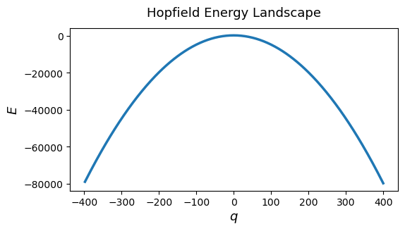
This clearly demonstrates that the Hebbian learning rule actually forms two energy minima, one of which is at the inverse of the original memory. Now lets try some more advanced learning rules.
Spurious Minima
To start, we can extend the Hebbian learning rule to encode multiple memories at once. Rather than defining \(W_{ij} = S_i S_j\) how we did for a single memory, you can simply sum the different \(S_i S_j\) pairs together for the different memories, so \(W_{ij} = S^{(1)}_i S^{(1)}_j + S^{(2)}_i S^{(2)}_j + ...\)
def hebbian_weights(*memories):
    M = np.array(memories)
    W = M.T @ M
    np.fill_diagonal(W, 0)
    return W, np.zeros(M.shape[1])

def two_memory_dataset(S1, S2, W, B):
    agree = np.where(S1 == S2)[0]
    disagree = np.where(S1 != S2)[0]
    dataset = {"S": [], "q1": [], "q2": [], "E": []}
    for a in range(len(agree) + 1):
        for d in range(len(disagree) + 1):
            S = -S1.copy()
            S[agree[:a]] = S1[agree[:a]]
            S[disagree[:d]] = S1[disagree[:d]]
            dataset["S"].append(S)
            dataset["q1"].append(S @ S1)
            dataset["q2"].append(S @ S2)
            dataset["E"].append(compute_energy(S, W, B))
    return dataset

def plot_energy_landscape(dataset):
    q1 = np.asarray(dataset["q1"])
    q2 = np.asarray(dataset["q2"])
    E  = np.asarray(dataset["E"])
    fig, ax = plt.subplots(figsize=(8, 7))
    heatmap = ax.tricontourf(q1, q2, E, levels=50, cmap="viridis")
    minima = np.isclose(E, E.min())
    ax.scatter(q1[minima], q2[minima], s=70, c="red", marker="o")
    fig.colorbar(heatmap, ax=ax, label=r"$E$")
    ax.set_xlabel(r"$q_1$", fontsize=14)
    ax.set_ylabel(r"$q_2$", fontsize=14)
    ax.set_title("Hopfield Energy Landscape", fontsize=15)
    plt.show()

S2 = np.array(Image.open("images/owl-20x20.png").convert("1"), dtype=int).flatten()
S2[S2==0] = -1
W, B = hebbian_weights(S, S2)
dataset = two_memory_dataset(S, S2, W, B)
plot_energy_landscape(dataset)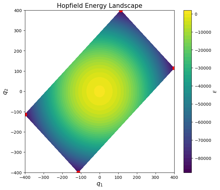
Here we can see that \(q_1=400\), \(q_1=-400\), \(q_2=400\), and \(q_2=-400\) are all minima (indicated by the red dots). These minima perfectly correspond to the two memories and the inverses of these memories. Now lets see what happens if you try and add even more memories.
S3 = np.array(Image.open("images/rocket-20x20.png").convert("1"), dtype=int).flatten()
S3[S3==0] = -1
W, B = hebbian_weights(S, S2, S3)
dataset = two_memory_dataset(S, S2, W, B)
plot_energy_landscape(dataset)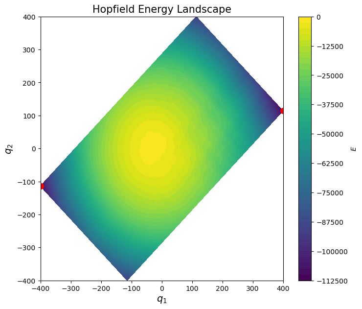
Here the results are slightly less promising. After adding a third memory to the weights, the second memory is no longer a global minima. It is still a local minima as far as we can see in this plotted region. Lets try plotting a few different regions.
dataset = two_memory_dataset(S, S3, W, B)
plot_energy_landscape(dataset)

dataset = two_memory_dataset(S2, S3, W, B)
plot_energy_landscape(dataset)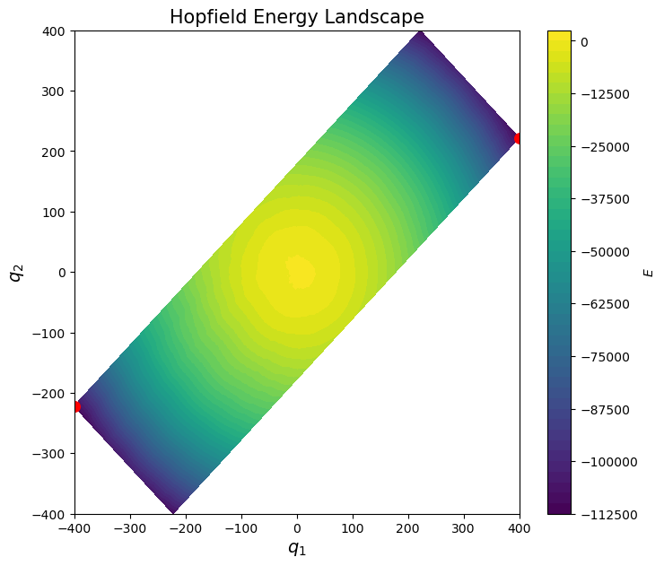
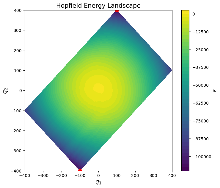
Based on these plots, it seems like after adding a third dimension, the memories are no longer strict global minima. Are there any other global minima in this new energy landscape? Consider \(S_{\text{spur}} = \text{sign}(S_1 + S_2 + S_3)\). Lets try plotting this memory using the existing weights.
S_spur = np.sign(S + S2 + S3)
dataset = two_memory_dataset(S, S_spur, W, B)
plot_energy_landscape(dataset)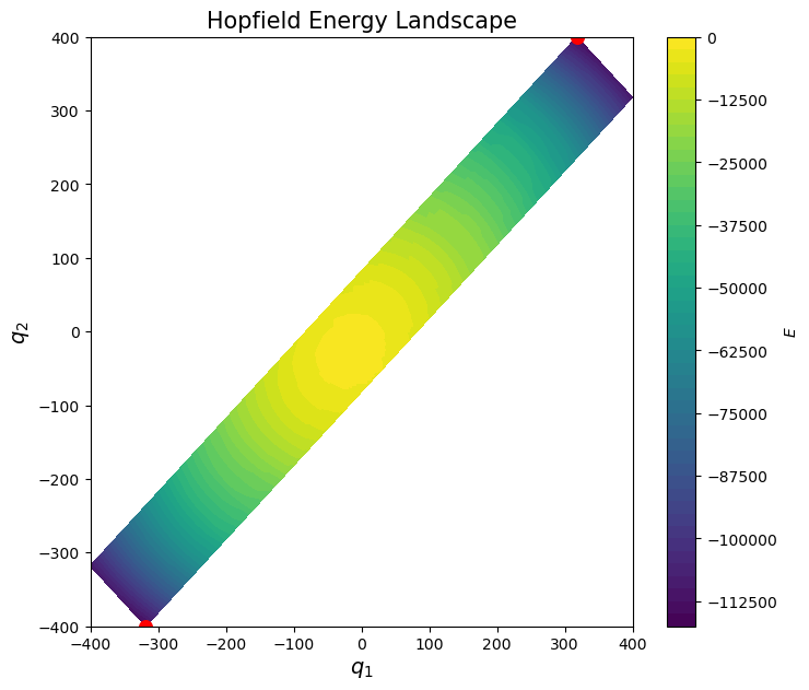
Now the issue is clear. \(S_{spur}\) has turned into a spurious minima, or an extra memory that got encoded into the weights. This memory seems to have a lower minima than \(S_1\), so random images would converge toward this unwanted memory rather than towards \(S_1\). This is a fundamental limitation of the Hebbian learning rule. Boltzmann machines are a much more powerful extension of Hopfield nets that can help deal with this issue.